Understanding Transformer Mechanisms Through a Toy Model

A Transformer does not initially “understand context.” It first learns a bigram statistics table, then learns to move information carried by distant tokens to the current position. Only then does it learn what information the current prediction needs, and which earlier token to ask for it.

We have heard plenty of metaphors for Q, K, and V: Query is the question, Key is the index, and Value is the content. Attention is compared to search, databases, and libraries.

These metaphors are not necessarily wrong, but they skip the truly interesting question:

Why does gradient descent train Q, K, and V to take on these roles?

Without an answer, “Q is a query and K is a key” merely restates how the formula operates. It does not explain the mechanism.

The ICLR 2026 paper How Do Transformers Learn to Associate Tokens: Gradient Leading Terms Bring Mechanistic Interpretability offers a rare and remarkably elegant answer. Starting from a three-layer attention-only toy model, the authors expand early-training gradients into leading terms and obtain approximate closed-form solutions for each parameter group. Instead of unreadable higher-order tensors, the result involves three simple corpus statistics:

• Bigrams: what typically follows a token.
• Interchangeability: which tokens fit similar functional slots.
• Context: what typically appears in the longer prefix before a token.

Better still, these statistics do not enter the model in parallel. Following the order in which gradients can propagate, they develop into output, value, and query-key attention:

$$W_O=O(\eta), \qquad V=O(\eta^2), \qquad W_{QK}=O(\eta^4).$$

This yields a more accurate picture of attention than “looking things up in a dictionary”:

Value defines the predictive correction a historical token can supply. Query-Key defines how much the current token needs that correction. Attention matches supply with demand; Value delivers the actual information after the match.

Below, we derive this story from the equations, then test it with a three-layer model we trained on TinyStories.

---

1. Shrinking the model until we can see through it

The paper studies an attention-only Transformer rather than a full GPT, retaining the causal mask, residual stream, and relative positional encoding. Input tokens are represented directly as one-hot vectors in vocabulary space:

$$X\in\mathbb R^{T\times |\mathcal V|}.$$

Layer $l$ is written as:

$$A^{(l)} = \operatorname{softmax}\!\left( \operatorname{Mask} \left[ h^{(l-1)}W^{(l)}h^{(l-1)\top} +D\!\left(P^{(l)}\right) \right] \right),$$ $$h^{(l)} = h^{(l-1)} +A^{(l)}h^{(l-1)}V^{(l)}, \qquad h^{(0)}=X,$$

The final output logits are:

$$F_\Theta(X)=h^{(L)}W_O.$$

One detail needs to be clear from the outset: the paper directly analyzes the combined query-key matrix $W^{(l)}$. In a standard Transformer, this corresponds to a combination of $W_QW_K^\top$. The individual $Q$ and $K$ have freedom under changes of basis. Their product is what determines attention scores, making it more identifiable.

We therefore discuss “what QK learns,” without pretending that scores alone uniquely explain a particular column of $W_Q$ or $W_K$.

This model has no MLP, LayerNorm, or the high-dimensional embeddings of mature LLMs. It cannot explain every capability of Transformers. It does, however, preserve the causal chain we care about:

$$\text{historical token} \xrightarrow{V} \text{message} \xrightarrow{attention} \text{current position} \xrightarrow{W_O} \text{next-token logits}.$$

Because the model is small enough, gradient expansions can illuminate this chain directly for the first time.

---

2. Zero initialization as an X-ray of training dynamics

Suppose all parameters start at zero, and we use gradient descent with cross-entropy loss and learning rate $\eta$.

Two things happen at initialization:

1. $W_O=0$, so every next-token logit is zero and predictions are uniform.
2. $W^{(l)}=P^{(l)}=0$, so causal attention averages uniformly over all visible prefix positions.

The point is not whether zero initialization is suitable for modern LLM training. It temporarily breaks the coupling between parameters, letting us observe when each gradient pathway first becomes active.

To keep the closed-form solutions from seeming to appear out of nowhere, let us retain a minimal gradient map. We write only one layer below; under zero initialization, all layers share the same leading term.

Let $Y_i$ be the next-token one-hot labels, let $S_i=\operatorname{softmax}(F_i)$, and define the residual measuring how much the model still owes the labels:

$$R_i=Y_i-S_i.$$

Ignoring common constants and summation signs, the chain rule has this structure:

$$\begin{aligned} \nabla_{W_O}\mathcal L&\propto-H^\top R,\\ \nabla_V\mathcal L&\propto-X^\top A^\top RW_O^\top,\\ \nabla_W\mathcal L&\propto-X^\top\mathcal J_A \!\left[RW_O^\top V^\top X^\top\right]X. \end{aligned}$$

$\mathcal J_A$ is the row-wise Jacobian of the attention softmax. These three lines already reveal the order: $W_O$ does not depend on $V$; $V$ must pass through $W_O$; and QK must pass through both $V$ and $W_O$.

2.1 Step one: only the output matrix can move

Initially, $V=0$, so $H_i=X_i$. Since $W_O=0$, all logits are zero, and $S_i$ is the uniform distribution $U$ over the vocabulary. Substituting into the first gradient pathway:

$$\frac{\partial \mathcal L}{\partial W_O} = -\frac{1}{NT} \sum_{i=1}^{N} X_i^\top(Y_i-U).$$

Define the centered bigram matrix $\bar B$:

$$\bar B_{ij} = P_t(e_i)P_t(e_j\mid e_i) -\frac{P_t(e_i)}{|\mathcal V|}.$$

There is no hidden step here: $(X_i^\top Y_i)_{jk}$ counts transitions $e_j\to e_k$ in the sequence. Averaging over data and positions turns the first term into the joint bigram frequency; $(X_i^\top U)_{jk}$ is the current-token frequency multiplied by the uniform probability. Their difference is exactly $\bar B$.

After the first update:

$$\boxed{W_O^{(1)}=\eta\bar B.}$$

The meaning is simple: if the current token is $e_i$, then $e_iW_O$ describes the shift of its average next-token distribution away from the uniform baseline.

The model’s first capability is not contextual understanding, but a statistical continuation table:

in   → the
was  → a
one  → day
.    → he / the

Why do $V$ and QK remain unchanged? When $W_O=0$, even if the attention block generates information, no decoder can read it into logits. With the downstream readout still zero, the upstream information-transport system receives no learning signal.

2.2 Step two: Value learns how history can change a prediction

After step one, $W_O$ can already decode hidden states into bigram logits. Changing the message sent by a historical token can now change the loss, activating the value gradient for the first time.

QK is still zero, so causal attention remains the fixed uniform matrix $A_0$: the first $t$ positions of row $t$ are all $1/t$, and future positions are zero. We also have:

$$W_O=\eta\bar B, \qquad R_i=(Y_i-U)+O(\eta).$$

Substitute these into the gradient of $V$ and retain the lowest-order term:

$$\nabla_V\mathcal L \approx -\eta \left[ \frac1{NT}\sum_i X_i^\top A_0^\top(Y_i-U) \right] \bar B^\top.$$

Why is the bracketed expression a context mapping? $A_0$ takes a contribution of $1/t$ from each token before position $t$; $X_i^\top$ then aggregates by token identity. Its $(j,k)$ element is therefore the average proportion of $e_j$ in the prefix when the target is $e_k$, minus the uniform-output baseline:

$$\frac1T\sum_t\frac1t\sum_{m\le t} P(x_{t+1}=e_k,x_m=e_j) -\text{uniform centering}.$$

This is exactly $\bar\Phi^\top_{jk}$. The second gradient-descent update is therefore:

$$V^{(2)} \approx \eta^2\bar\Phi^\top\bar B^\top.$$

If training continues for $s$ steps, $W_O$ is approximately $r\eta\bar B$ before step $r$. The leading term written into $V$ at each step is consequently proportional to $r\eta^2$, and:

$$\sum_{r=0}^{s-1}r=\binom{s}{2}.$$

The paper’s general expression is thus not a guess, but the result of accumulating gradients at each step:

$$\boxed{ V^{(l)} \approx \binom{s}{2}\eta^2 \bar\Phi^\top\bar B^\top }$$

The full definition of $\bar\Phi$ can be written as:

$$\bar\Phi_{ij} = \frac1T \sum_{k=1}^{T} \frac1k \sum_{m=1}^{k} P(x_{k+1}=e_i,x_m=e_j) -\mu_j.$$

$\bar\Phi_{ij}$ measures how likely $e_j$ is to appear in the preceding prefix when the current or target token is $e_i$.

For example, in TinyStories:

fish  ← pond / water / whale / fisherman
birds ← tree / park / bird

Attention scores are still close to uniform. Yet uniform averaging already lets $V$ learn its first long-range capability: what correction an earlier token should supply to later predictions.

Its order is $O(\eta^2)$, which can also be read directly from the computation graph:

$$\underbrace{W_O}_{O(\eta)} \times \underbrace{\eta}_{\text{this update}} =O(\eta^2).$$

This is more precise than “V stores content.” A better description is:

V learns the statistical correction a historical token can supply to the next-token distribution, in a form the output layer can read.

2.3 Step three: QK finally has a reason to choose whom to listen to

Transport alone is insufficient. Uniform attention mixes messages from all historical tokens. Only when:

• $V$ can produce meaningful messages, and
• $W_O$ can read those messages into logits,

can changing attention scores have a first-order visible effect on the loss.

The QK gradient pathway must therefore contain at least:

$$\underbrace{V}_{O(\eta^2)} \times \underbrace{W_O}_{O(\eta)} \times \underbrace{\eta}_{\text{this update}} =O(\eta^4).$$

The order tells us only when the effect appears. Substituting $W_O$ and $V$ back into the score gradient, and removing scale constants, gives the core dependence:

$$R_iW_O^\top V^\top X_i^\top \ \propto\ (Y_i-U) \underbrace{\bar B^\top\bar B}_{\Sigma_{\bar B}} \bar\Phi X_i^\top.$$

This measures how useful the information at each prefix position is for correcting a next-token prediction. The softmax Jacobian at the uniform point then removes future positions and subtracts the row mean over the visible prefix.

This centering is revealing: attention can learn only who is more worth listening to than the average historical token. Adding the same constant to every key does not change the softmax.

Call this row-wise masked-and-centered result $Q_i$. Since the label at row $t$ of $Y_i$ is $x_{t+1}$, it also performs a natural next-to-query alignment: evidence found for predicting $x_{t+1}$ is written into the score whose query is the current token $x_t$.

Finally, use the one-hot vectors $X_i$ on both sides to aggregate position pairs into vocabulary-level query-key token pairs:

$$\boxed{ \bar Q = \frac1{NT}\sum_i X_i^\top Q_iX_i. }$$

Thus, $\bar Q_{ab}$ does not mean “$a$ and $b$ often co-occur.” It asks whether, when the current query is $a$, attending to historical token $b$ can improve the prediction through the pathway “context $\to$ interchangeable candidates $\to$ next token.”

The coefficient also has a simple origin. Before update $r+1$, $W_O$ has accumulated $r$ contributions, and $V$ has accumulated $\binom r2$ contributions. The QK coefficient for this update is therefore $r\binom r2$. Summing over training steps gives the leading term:

$$\boxed{ W^{(l)} \approx \left[ 3\binom{s}{4} +2\binom{s}{3} \right] \eta^4\bar Q. }$$

This combinatorial coefficient equals 2 at $s=3$, reducing exactly to the third-step result above. The full proof must also control softmax linearization error and higher-order parameter remainders. These determine how long the approximation holds in early training, without changing the mechanism’s chain of dependencies.

Positional encoding $P^{(l)}$ appears at the same order, projecting the same predictive relevance onto relative positions rather than token pairs.

This training order is the most elegant part of the paper:

Order of appearance	Parameter	Initial function learned	Learning-rate order
1	$W_O$	Average continuation statistics of the current token	$O(\eta)$
2	$V$	The predictive correction a historical token can supply	$O(\eta^2)$
3	$QK$	Which historical token the current prediction should ask for a correction	$O(\eta^4)$

The model is not given predefined Q/K/V roles and then asked to fill in their parameters. These roles arise from the ordering of gradient dependencies in the computation graph.

---

3. How three corpus statistics combine into “semantics”

3.1 $\bar B$: rows and columns tell different stories

Row $r$ of $\bar B$ is a next-token predictive profile scaled by corpus frequency $P_t(e_r)$: given current token $e_r$, which outputs are more likely than the uniform baseline?

in   → the
fish → swam / swimming
.    → he / the

But it is the columns that enter the Gram matrix. Denote column $i$ by:

$$b_i:=\bar B_{:,i}.$$

$b_i$ collects predictive evidence from all possible predecessors for candidate token $e_i$. If $b_i$ and $b_j$ are similar, $i,j$ are predicted by similar predecessors in similar ways, allowing them to occupy similar linguistic slots.

For example, happy/sad/excited/scared all commonly follow she was .... They are not necessarily synonyms, but have similar predictive roles. What is learned here is functional interchangeability, not semantic categories from a human dictionary.

3.2 $\bar B^\top\bar B$: similarity is only half the story

The paper interprets:

$$\Sigma_{\bar B}=\bar B^\top\bar B$$

as an interchangeability mapping, because:

$$(\Sigma_{\bar B})_{ij}=b_i^\top b_j.$$

But an inner product is not pure cosine similarity. Let:

$$d_i=\lVert b_i\rVert_2, \qquad D=\operatorname{diag}(d_1,\ldots,d_{|\mathcal V|}),$$

and let $C_{ij}=\cos(b_i,b_j)$; define cosine as zero for zero-norm columns. We then obtain an exact decomposition:

$$\boxed{ \bar B^\top\bar B=DCD. }$$

The paper uses interchangeability to interpret this Gram matrix. $DCD$ is an equivalent rewriting used here to separate “evidence strength” from “role similarity,” not an additional assumption.

Here, $C$ is pure role similarity, while $D$ measures the predictive statistical strength of the two endpoints. A more accurate name for $\bar B^\top\bar B$ is therefore:

Functional similarity weighted by statistical evidence.

$d_i$ is not just word frequency. By the definition of $\bar B$:

$$d_i^2 = \sum_r P_t(e_r)^2 \left[P_t(e_i\mid e_r)-\frac1{|\mathcal V|}\right]^2.$$

It incorporates how common the predecessors are, how strongly their predictions deviate from the uniform baseline, and how many predecessors jointly support $e_i$. Direction answers “what role does it play?” Norm answers “how much corpus evidence supports that role?”

This also explains why cosine alone is insufficient. Even if a rare token happens to point in the same direction as fish, a small $d_i$ prevents it from inheriting all of fish’s evidence.

3.3 $\bar\Phi$: a context token’s candidate list

$\bar\Phi$ goes beyond direct adjacency to summarize long-range prefixes. Given historical token $e_k$, define:

$$\phi_k:=\bar\Phi_{:,k}.$$

$\phi_k$ is a future-token association list: entry $j$ records how much direct statistical support future token $e_j$ receives when $e_k$ appears earlier in the text.

For example, if the corpus frequently contains pond ... fish, then $\bar\Phi_{\text{fish},\text{pond}}>0$. This is a direct long-range association; the evidence has not yet been generalized to functionally similar tokens such as frog.

3.4 $\bar B^\top\bar B\phi_k$: similarity propagation with statistical support

Now pass context evidence through the interchangeability kernel:

$$g_k = \bar B^\top\bar B\phi_k = DCD\phi_k.$$

Its $i$ entry can be expanded fully:

$$\boxed{ (g_k)_i = d_i\sum_j C_{ij}\,d_j\,\bar\Phi_{jk}. }$$

Read this multiplication from right to left:

1. $\bar\Phi_{jk}$: context $k$ directly supports candidate $j$.
2. $d_j$: how reliable that candidate’s evidence is.
3. $C_{ij}$: propagate the evidence to $i$, whose predictive role is similar.
4. $d_i$: whether recipient $i$ has enough statistical support of its own.

Suppose pond directly supports fish, but hardly supports frog directly:

$$\bar\Phi_{\text{fish},\text{pond}}=0.8, \qquad \bar\Phi_{\text{frog},\text{pond}}\approx0.$$

If $d_{\text{fish}}=0.9$ and $d_{\text{frog}}=0.7$, and their role cosine is $0.95$, the indirect contribution propagated from fish to frog is approximately:

$$0.7\times0.95\times0.9\times0.8 \approx0.48.$$

The model can thus generalize the observed pond → fish association into pond → frog, even though the latter is less frequently observed directly. Cosine determines where to generalize; the $D$ factors on both sides determine how much evidence and support are available for generalization.

If $C_{ij}<0$, this pathway can transmit inhibition rather than support. It is therefore not probability diffusion, but signed kernel propagation weighted by evidence strength.

“Semantics” here is no mysterious extra object injected into the model. It is a strength-weighted propagation of long-range co-occurrence evidence along functional similarity.

---

4. Why attention is supply-demand matching

4.1 $\bar\Phi^\top\bar B^\top$: encoding output wishes into hidden messages

The leading term of Value is:

$$V\propto\bar\Phi^\top\bar B^\top.$$

Given historical token $e_k$, the first step:

$$e_k\bar\Phi^\top=\phi_k^\top$$

lists the future tokens it wants to promote or suppress. Think of this as an “output wish list.” But a value vector lives in hidden space; the list cannot simply be inserted into the logits.

The second step therefore multiplies by $\bar B^\top$:

$$v_k=e_kV=\phi_k^\top\bar B^\top.$$

In this toy model, the hidden basis coincides with the token basis. Its $r$ hidden coordinate is:

$$(v_k)_r = \sum_j\bar\Phi_{jk}\bar B_{rj} = \langle\phi_k,\bar B_{r,:}\rangle.$$

In other words, it searches for hidden basis vectors that, when decoded by the output layer, can produce the candidate list. $\bar B^\top$ is not an inverse here, but the adjoint of the output layer: a matched-filter-like back-projection.

We can therefore read $\bar\Phi^\top\bar B^\top$ as:

First decide what a historical token wants to say to the output, then encode that statement as a hidden message the output layer understands.

4.2 What happens when the message reaches the logits?

The raw value message must ultimately pass through $W_O\approx\bar B$:

$$m(e_k) = e_k\bar\Phi^\top\bar B^\top\bar B = \phi_k^\top\Sigma_{\bar B} = g_k^\top.$$

This is exactly the evidence-weighted similarity propagation from the previous section, expressed using the forward pass’s row-vector convention.

Expression	What it does
$\phi_k=\bar\Phi_{:,k}$	The direct candidate list supplied by context $k$
$\phi_k^\top\bar B^\top$	Encodes the candidate list into a hidden message
$\phi_k^\top\bar B^\top\bar B$	The message’s actual effect on logits after decoding

“V stores token content” is therefore too static a description. Here, V resembles a compiler: it compiles long-range context evidence into predictive corrections that the current output system can execute.

Substitute the leading terms back into a single-layer model, ignoring scale constants:

$$F(X) \approx \underbrace{X\bar B}_{\text{local bigram baseline}} + \underbrace{A(X)X\bar\Phi^\top\Sigma_{\bar B}}_{\text{long-range generalizable correction}}.$$

4.3 QK: does the current prediction need this supply?

Every historical token can produce a message, but not every position should receive it. QK learns the compatibility between a message and the current prediction’s shortfall.

The score of current query $e_q$ for historical token $e_k$ is:

$$s(q,k) = e_q\bar Qe_k^\top+\Delta_{q-k}.$$

The formation of $\bar Q$ can be understood in three steps:

1. Use the true next-token residual to assess whether the logit message from $e_k$ can reduce the current error.
2. Apply the causal mask to exclude the future, then compare against average usefulness in the current prefix.
3. Write the result into the vocabulary coordinates of the current query token and historical key token.

QK therefore learns more than token similarity in the general sense. It asks:

When query $q$ is about to predict the next token, is the correction supplied by historical token $k$ exactly what it currently needs?

This is attention’s supply-demand interpretation:

• Query expresses what the current prediction lacks.
• Key identifies the kind of evidence a historical position can offer.
• The QK score measures the match between demand and supply.
• Value encodes the successfully matched evidence into a hidden message.
• $W_O$ decodes the message, generalizing along statistically reliable functional similarities.

“Q and K perform retrieval” describes the operation. “Supply-demand matching” explains why next-token loss trains them to retrieve these particular things.

---

5. How we reproduced this story

Based on the authors’ open-source implementation, we reproduced the first TinyStories stage of the paper and made numerically equivalent memory-saving changes for a shared A800.

Experimental configuration:

Setting	Value
Model	3-layer attention-only Transformer
Vocabulary	The 3,000 most common natural-word tokens in TinyStories
Training sequences	65,536
Sequence length	200
Initialization	Zero initialization
Optimizer	SGD
Learning rate	0.005
Effective batch size	2,048
Samples for theoretical statistics	2,048
Training	10 epochs

To preserve the effective batch size, we used micro-batches of 256 with eight gradient-accumulation steps. Dense one-hot multiplications for the theoretical matrices were rewritten as numerically equivalent sparse counting operations. The complete configuration and code are in the MergeOpt repository.

5.1 The closed-form directions really appear in the weights

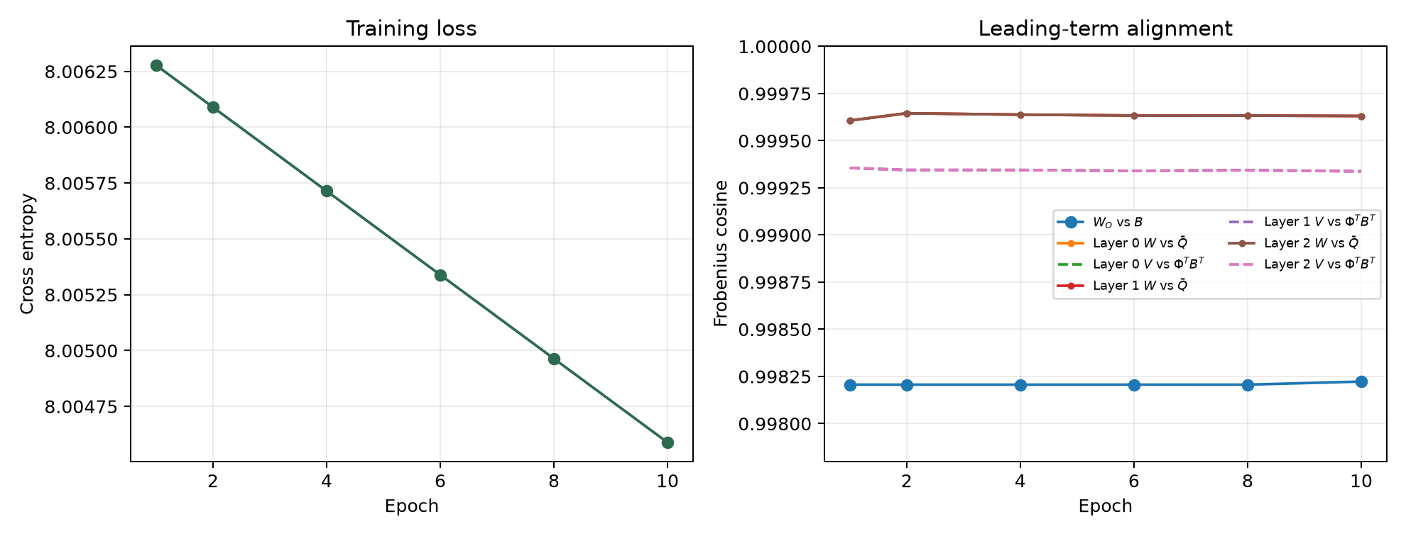
At epoch 10:

Alignment	Frobenius cosine
$W_O$ vs. $\bar B$	0.998223
$V$ vs. $\bar\Phi^\top\bar B^\top$	0.999337
QK matrix vs. $\bar Q$	0.999631

The curves of all three layers also almost coincide. This matches the theory: near zero initialization, layers begin with the same corpus-level associative basis. Specialization between layers appears only after higher-order terms accumulate.

But do not yet interpret a cosine near 1 as “the mechanism is already working strongly.” As we will see, direction and behavior are different things.

5.2 Three very different kinds of association for the same token

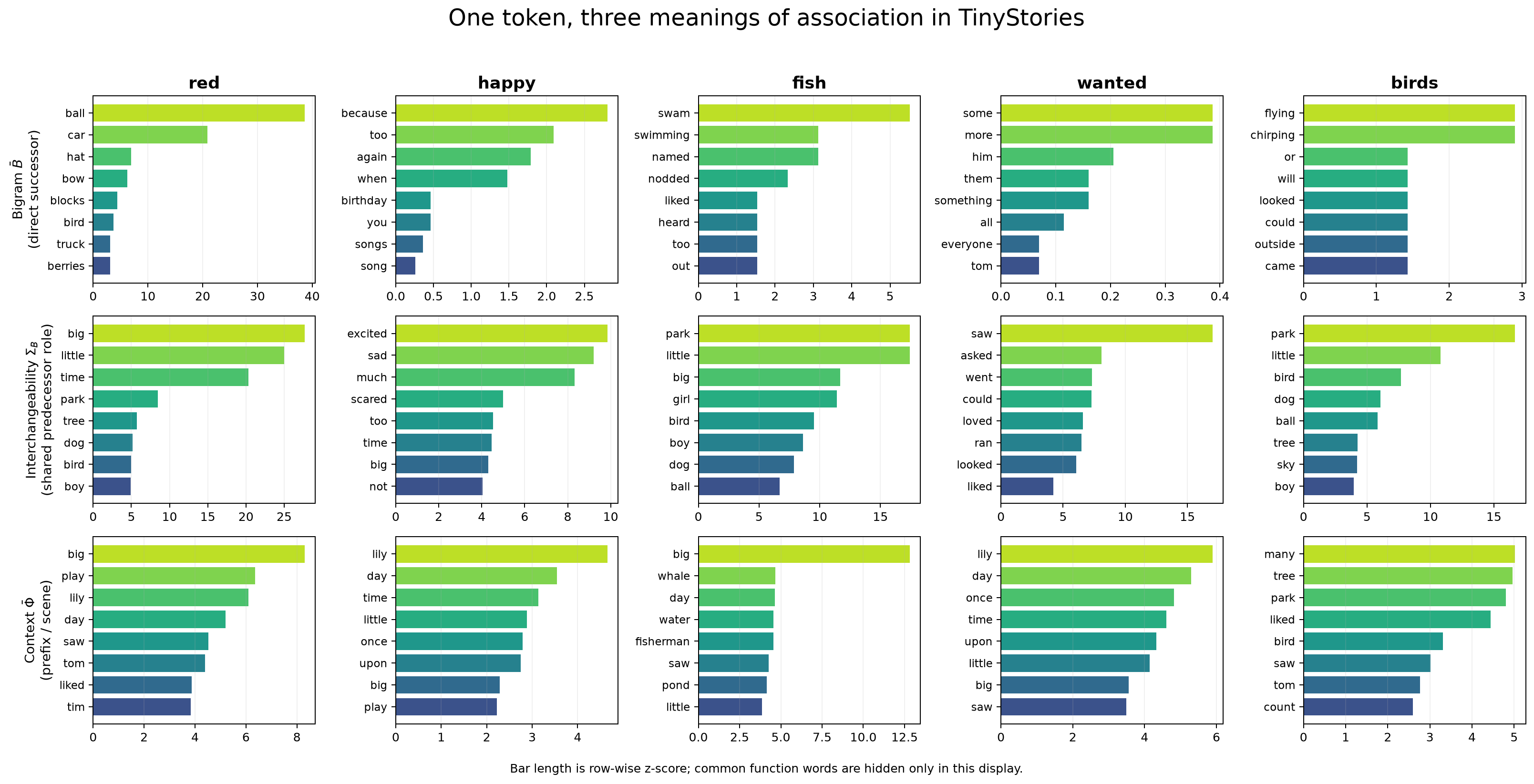
Each column above represents an anchor token; the three rows show its neighbors under bigram, interchangeability, and context mappings.

Take fish as an example:

Bigram:             swam / swimming / named
Interchangeability: park / little / big / girl / bird
Context:            whale / water / fisherman / pond

This is a useful reminder not to call every co-occurrence “semantic similarity”:

• fish → swam is a compositional collocation.
• fish ↔ bird/girl mostly reflects interchangeability in templates and grammatical roles.
• fish ← pond/water comes closer to our intuitive notion of scene knowledge.

On a small manually constructed category probe, the same-category Top-10 hit rate of $\Sigma_{\bar B}$ reaches 42.2% for emotions, 17.8% for motion, and 16.4% for animals, but 0% for colors. The reason is straightforward: emotion words strongly share the was ___ template, while colors often share adjective slots with big/little.

The model learns functional geometry in the data, not an ontology predefined by humans.

5.3 How context is activated in a real story

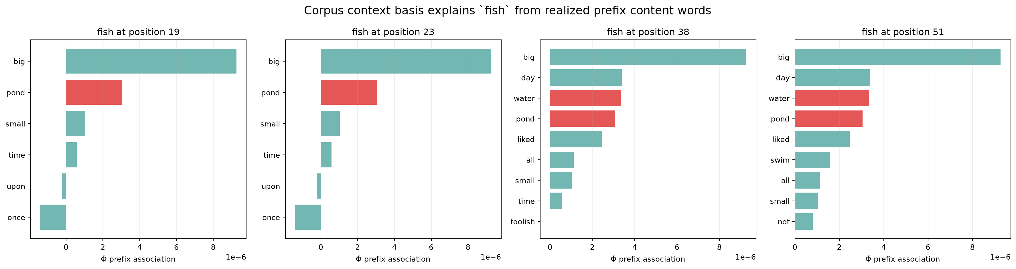
We selected a real story from TinyStories:

once upon a time, there was a small pond. in the pond, there was a big fish …

For fish at positions 19, 23, 38, and 51, we searched for $\bar\Phi$ evidence only among content words that had actually appeared earlier in that story.

Early occurrences of fish already receive corpus-level support from pond. Once water appears later in the story, it joins the explanatory set for subsequent occurrences of fish. What happens here is:

$$\text{global corpus pond--fish statistics} \times \text{pond appears in the current sample}.$$

This is a minimal prototype of the transition from corpus statistics to conditioned behavior.

5.4 Output first learns the skeleton of language

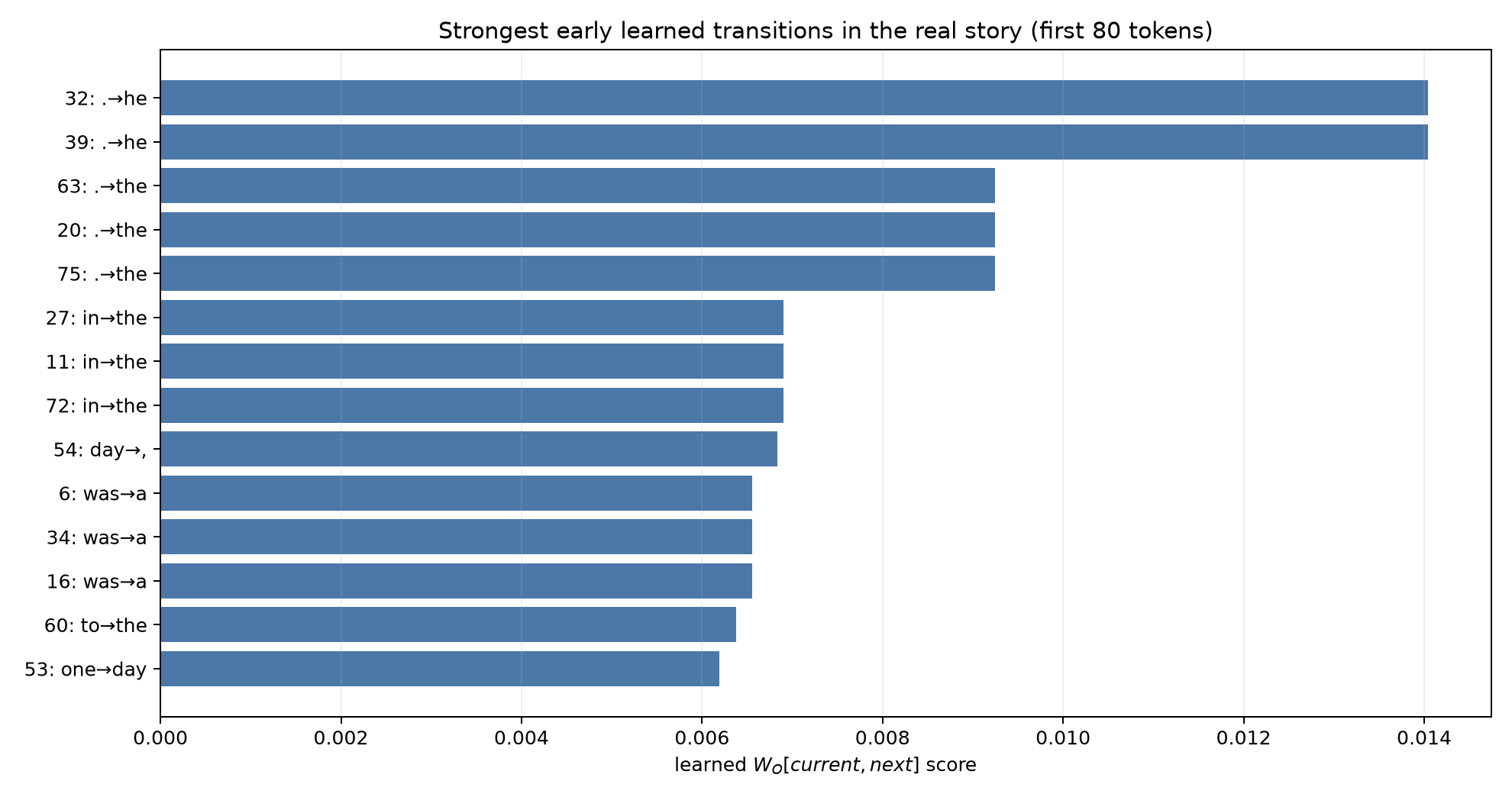
Among the first 80 tokens of the story, the real transitions most strongly supported by learned $W_O$ include:

.   → he
.   → the
in  → the
day → ,
was → a
one → day

These are not complex story comprehension, but a linguistic skeleton made of prepositions, articles, punctuation, and recurring TinyStories openings.

For example, . → he:

$$W_O[\texttt{.},\texttt{he}]\approx0.0140, \qquad \bar B[\texttt{.},\texttt{he}]\approx0.00895.$$

The absolute values need not match, because the closed-form solution also includes coefficients for training steps and learning rate. What matters is the strong agreement in matrix direction and relative structure.

---

6. The strangest result: the parameters “understand,” but behavior has not begun

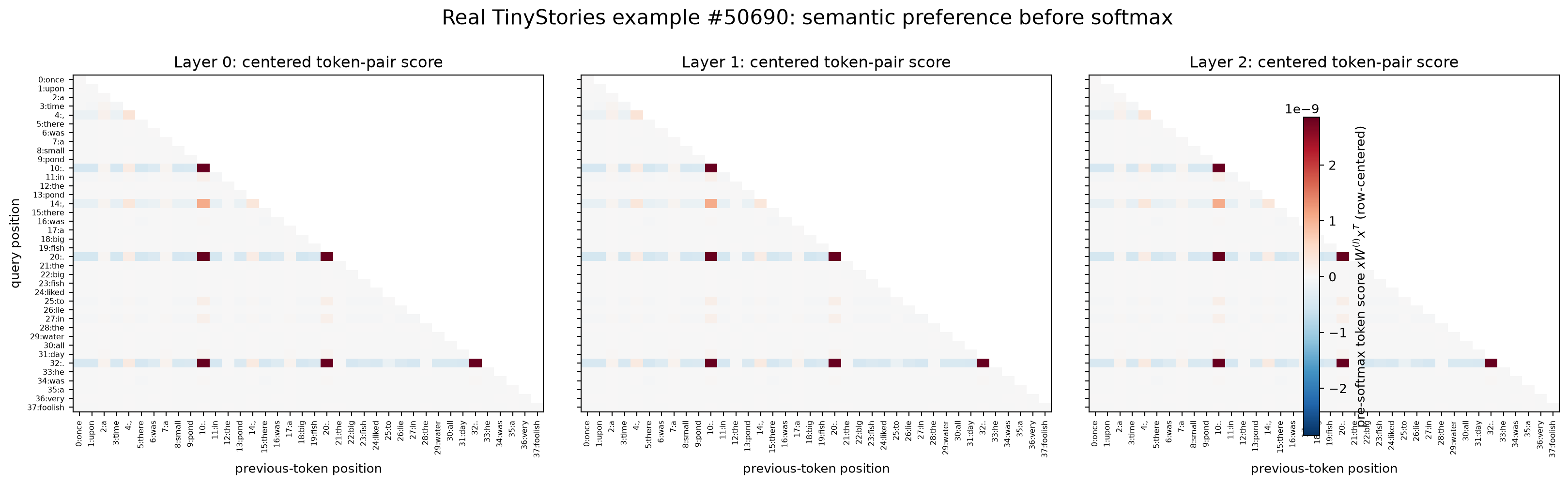
The figure shows pre-softmax, row-centered token-pair scores from the three layers on a real story:

$$XW^{(l)}X^\top.$$

They have a stable structure and are almost identical across layers. Yet the scale of the scores is only about $10^{-9}$. In float32:

$$\operatorname{softmax}(z+10^{-9}\epsilon) \approx \operatorname{softmax}(z),$$

The maximum visible change in actual attention probabilities relative to uniform causal attention is zero.

In other words:

$$\boxed{ \text{cosine of QK with theoretical direction}=0.9996 \quad\not\Rightarrow\quad \text{attention already affects behavior} }$$

For a causal check, instead of indiscriminately zeroing out entire layers, we removed only the learned weights’ projection onto the theoretical leading term $T$:

$$W' = W- \frac{\langle W,T\rangle_F}{\|T\|_F^2}T.$$

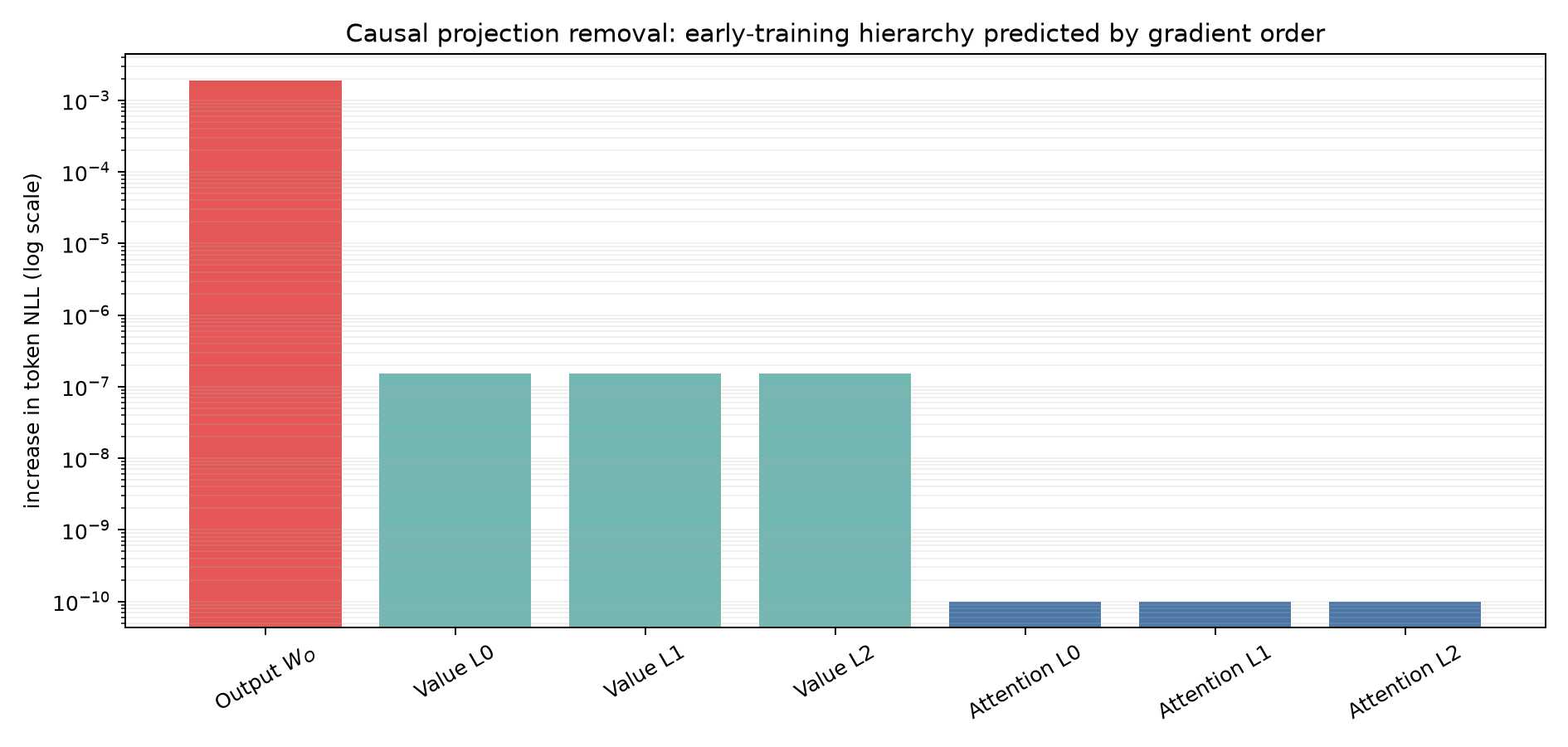
Results on 64 samples:

Removed component	$\Delta$ token NLL
Output $\bar B$	$1.91\times10^{-3}$
Value leading term in each layer	$1.53\times10^{-7}$
Attention $\bar Q$ in each layer	Zero at the current numerical precision

This reproduces exactly the behavioral hierarchy predicted by the gradient orders:

$$O(\eta) \gg O(\eta^2) \gg O(\eta^4).$$

The paper performs similar ablations on a more extensively trained model with a higher learning rate. The original loss is 5.349; removing the output leading term increases it to 8.287; removing value increases it to approximately 6.19–6.53; removing attention leading terms in the three layers increases it only to 5.350–5.361. The paper’s appendix shows the same ordering, with value already having a real effect in later training.

This is an important warning for mechanistic interpretability:

An interpretable parameter direction does not necessarily have a measurable causal effect yet.

Probes, cosine similarities, and attractive heatmaps tell us that a structure is present. Interventions and behavioral evaluations tell us whether the model is using it.

---

7. A less pretty, more realistic result: composition also amplifies template bias

The paper’s core feature composition for QK is:

$$\Sigma_{\bar B}\bar\Phi.$$

It first maps a token to a group of functionally similar tokens, then aggregates their shared long-range contexts. We decomposed this pathway for fish:

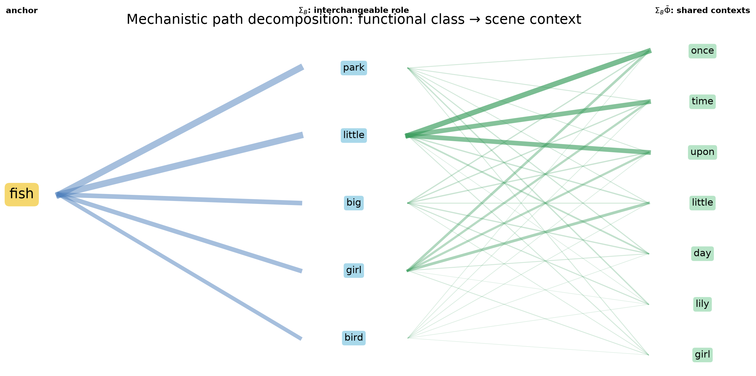
The strongest intermediate “interchangeable roles” are not purely an animal category, but:

park / little / big / girl / bird

After passing through the context mapping, the strongest shared contexts become:

once / time / upon / little / day / lily / girl

This is less aligned with human expectations of semantics than fish ↔ pond/water, but closely matches TinyStories templates:

once upon a time ...
one day ...
a little girl ...

This is not a failure of the theory. It is where the theory’s explanatory power is most honest. Matrix composition propagates statistical structure in the training corpus, not “truth.” It propagates semantics, but also templates, word frequency, and bias.

Emergence does not guarantee abstractions we like. It only means that local statistics, through reusable computational structures, can produce new conditioned functions.

---

8. From a shared starting point to layer specialization: interpreting later drift

In our low-learning-rate, 10-epoch reproduction, the three layers are almost identical. This does not mean that every layer has learned equally strong semantics. They are still in a phase dominated by a shared leading term.

The paper also analyzes different training checkpoints of Pythia-1.4B, which includes MLPs and multi-head attention. The authors transform each layer’s token representations and average QK mapping into the token basis, then compare them with leading-term covariances estimated from OpenWebText and FineWeb. The results show that early checkpoints align strongly with theoretical associative features, after which different layers gradually drift and attention heads specialize at different rates. Head variance in intermediate layers grows especially early. Pythia is well suited to this research because it releases densely spaced training checkpoints.[4]

We can interpret this as:

$$\text{shared statistical bootstrap} \longrightarrow \text{layer and head specialization} \longrightarrow \text{richer representations and capabilities}.$$

But restraint is necessary. Drift alone shows only that the model has left a fixed early associative basis. It is consistent with the development of richer knowledge and higher-level capabilities, but cannot by itself prove that drift caused a particular reasoning ability.

A more precise statement is:

Leading-term theory explains the shared foundation before higher-level capabilities develop. Drift marks where this simple explanation starts to break down and the model begins to specialize.

This is not an embarrassing boundary of the theory. It is the natural starting point for the next stage of mechanistic research: how much of the statistical foundation do later components retain, and what new composable structures do they add?

---

9. The Transformer intuition this toy model actually teaches

We can now condense the story into three statements.

9.1 $W_O$: first learn the average world

The current token directly looks up its average next-token distribution. This is a local statistical capability and the earliest visible skeleton of language.

9.2 $V$: let the past change the present

A historical token becomes more than a token ID. It maps to a set of predictive corrections the output layer can read, bringing long-range context and functional interchangeability into the current logits.

9.3 QK: retrieve the right past only when needed

The current query values historical tokens’ messages according to its own next-token needs. Key is not a static label: it becomes meaningful only relative to a particular query’s demand.

Attention therefore does more than “mix all the information” or “find similar tokens.” It performs:

$$\boxed{ \text{current predictive demand} \times \text{historical information supply} \rightarrow \text{conditioned logit correction} }$$

This also explains why bigram statistics alone are still memorization, while the combination of $V+$QK starts to look like generalization: the same historical evidence can serve multiple functionally similar candidates, and the same query demand can be satisfied by different positions in different stories.

What is remarkable about Transformers is not the cleverness of the Q/K/V names. Through gradient descent, next-token loss spontaneously expands a statistical lookup table into an information transporter, and then into a router that responds to demand.

---

10. What this model still cannot explain

The paper and our reproduction explain the early foundation of capability formation, not a complete mental model of LLMs:

• The toy model works in vocabulary one-hot space, without standard learned embeddings.
• It has no MLP or LayerNorm, and directly parameterizes the combined QK matrix.
• The theory primarily concerns zero initialization or sufficiently small Gaussian initialization, within a sufficiently early training window.
• Early attention has extremely weak behavioral effects; this article explains how its directions begin to emerge.
• The Pythia experiments compare token-correlation covariances. They support extrapolating the theory to real LLMs, but do not prove full equivalence.

These clear boundaries make the toy model an excellent introduction to Transformers. It does not replace mathematics with anthropomorphic metaphors. It shows how a function develops step by step from corpus statistics, the computation graph, and gradient orders.

The next time someone says “Query is the question, Key is the index, and Value is the answer,” you can ask:

Why does training make them that way?

At least for the earliest stage of learning token associations in Transformers, we now have a fairly concrete answer.

---

References

1. Shawn Im, Changdae Oh, Zhen Fang, Sharon Li. How Do Transformers Learn to Associate Tokens: Gradient Leading Terms Bring Mechanistic Interpretability, ICLR 2026.
2. Authors’ open-source code: deeplearning-wisc/attn-dynamics-basis.
3. Ronen Eldan, Yuanzhi Li. TinyStories: How Small Can Language Models Be and Still Speak Coherent English?, 2023.
4. Stella Biderman et al. Pythia: A Suite for Analyzing Large Language Models Across Training and Scaling, ICML 2023.
5. Ashish Vaswani et al. Attention Is All You Need, NeurIPS 2017.
6. Catherine Olsson et al. In-context Learning and Induction Heads, 2022.