A Simple Analysis of OPD Gradients

A reasoning response may contain thousands of tokens, yet only a small number of positions drive most of the learning. Beyond the 80/20 Rule applies RLVR updates only at the highest-entropy 20% of positions, retaining nearly the performance of full-token updates on Qwen3-8B and improving it on larger models. 1% of Tokens Can Be Enough reduces the OPD supervision budget to 0.1%–1%, while still approaching or exceeding full OPD in several mathematical and medical reasoning settings. A few tokens can be enough: this is an empirical phenomenon worth explaining.

A related phenomenon appears in on-policy distillation (OPD): suppressing tokens that the student generates but the teacher does not support can produce substantial gains. After one token is suppressed, though, what happens to the other candidates? Do they move toward the teacher’s preferences, or reinforce the student’s existing preferences?

We ran diagnostics and experiments around these two questions. Our central claim is that softmax geometry already concentrates the effective update budget, and entropy selection identifies the same positions with large gradients; when negative feedback squeezes one token, competition among the remaining candidates further amplifies the student’s existing preferences. One determines where learning signals concentrate; the other determines how suppressing a candidate affects its competitors.

1. Why a Few Token Updates Can Be Enough

1.1 A Few Tokens Carry Most of the Effective Update Budget

Fix a prefix and write the student distribution as $p=\operatorname{softmax}(z_\theta)$, with $y$ the generated token. Train this token with a detached scalar signal $A_y$:

$$\ell_y=-\operatorname{sg}(A_y)\log p_y.$$

In OPD, this signal is often the difference between the teacher’s and student’s log-probabilities for the same token. Write the score gradient as $g_y=\nabla_\theta\log p_y$. This token then contributes $A_y g_y$ to the raw gradient descent direction.

Softmax gives an important decomposition:

$$g_y=(1-p_y)h_y, \qquad h_y=\nabla_\theta\log\frac{p_y}{1-p_y}.$$

Here, $h_y$ is the gradient of the token’s log-odds against all remaining candidates. Before clipping and the optimizer, the length of its contribution is therefore

$$\boxed{\|A_y g_y\|=|A_y|(1-p_y)\|h_y\|.}$$

It depends on the learning signal, the student’s confidence, and the remaining gradient scale in parameter space. Even two tokens receiving the same signal can make vastly different contributions.

For example, $p_y=0.9990$ and $p_y=0.9999999934$ can both be described casually as “very confident.” Yet their $1-p_y$ values are $10^{-3}$ and $6.6\times10^{-9}$, a difference of roughly 150,000-fold. If the other factors are similar, their raw update budgets differ by roughly the same factor.

This geometry runs through both SFT and OPD: token cross-entropy uses the same score gradient. The supervision method determines the signal in front, while softmax determines its scale as it enters the model.

1.2 How Concentrated Is the Budget in Our Data?

Our initial diagnostic contained 8 short arithmetic rollouts, with 32 output tokens measured per response: 256 positions in total. We computed the full-parameter score norm at each position and obtained $1-p_y$ using the stable expression $-\operatorname{expm1}(\log p_y)$, avoiding loss of precision when subtracting probabilities close to 1.

Quantity	Result in this dataset
Range of the score norm $\|g_y\|$	$1.78\times10^{-12}$ to $1.99\times10^3$
5th / 50th / 95th percentiles of the residual norm $\|h_y\|$	491 / 1264 / 3138
Regression slope of $\log\|g_y\|$ against $\log(1-p_y)$	1.029
$R^2$ of that regression	0.9971

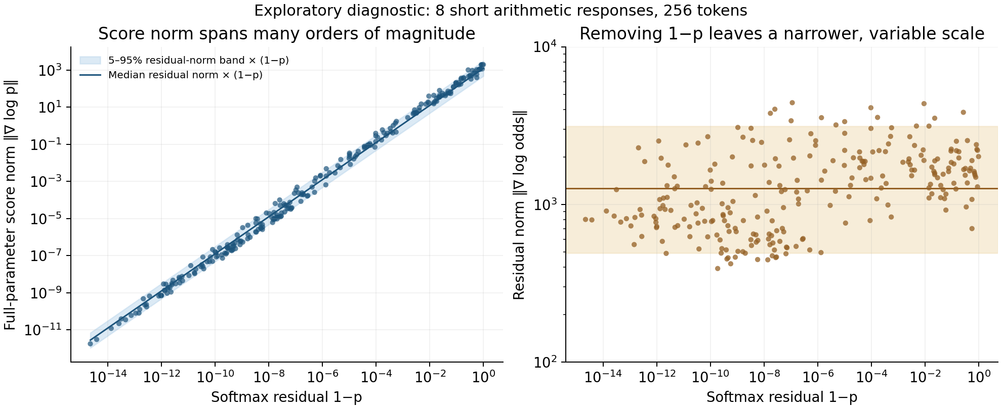
The score norm on the left spans about 15 orders of magnitude. After removing $1-p_y$, the central 90% interval of the residual norm on the right narrows to roughly a 6.4-fold range. In this dataset, $1-p_y$ is the main factor determining the gradient’s order of magnitude.

Only 28/256 positions, or 10.94%, have $p_y<0.9$, yet they account for:

• 92.52% of the sum of individual token score norms, which also describes the distribution of contribution lengths under a uniform negative signal.
• 97.14% of the actual teacher-gap-weighted contribution lengths, $\sum_y|A_y|\|g_y\|$.

Full-token training already implements an extremely uneven budget allocation: roughly 11% of positions take 97% of the teacher-gap-weighted contribution, with the rest sharing about 3%. From this perspective, sparse updates make an existing concentration explicit.

1.3 Entropy Selection Finds the Same Tokens with Large Gradients

We ranked positions by student entropy, sampled-token probability, and full-parameter score norm, then compared the highest-entropy, lowest-probability, and largest-norm sets. At the top-20% quantile threshold, each set contains 52 positions.

Comparison	Measured result
Overlap between highest entropy and lowest probability	52/52, 100%
Overlap between highest entropy and largest score norm	51/52, 98.08%
Score-norm budget retained by the highest-entropy set	99.27%
Teacher-gap-weighted budget retained by the highest-entropy set	99.21%

On these rollouts, the high-entropy selector is an almost exact selector for large gradients. High entropy, low probability, and large gradients describe the same positions that dominate updates. Selecting about 20% of tokens retains more than 99% of the budget: the selector captures the core positions that actually carry the learning.

This provides a direct optimization explanation for the role of high-entropy tokens. Low confidence keeps $1-p_y$ large enough for the learning signal to enter the model. High confidence drives this factor toward zero, leaving many positions almost silent during training. Entropy selection captures this difference and concentrates updates where the model actually responds.

We therefore argue that the importance of high-entropy tokens and the concentration of the gradient budget should be understood together. The 80/20 paper describes high-entropy positions as reasoning forks; our diagnostic explains them from the optimization side: their gradient scale gives them the overwhelming share of updates. Token-Level Analysis of Sampled-Token Reverse-KL OPD likewise decomposes the logit gradient into the teacher gap and $1-p_y$.

1.4 From 20% to 0.1%: Effective Updates Can Be Extremely Sparse

The 80/20 paper tests sparse updates in training: applying policy gradients only at the highest-entropy 20% of positions gives nearly full-update performance on Qwen3-8B and improves AIME’25 by 11.04 percentage points on Qwen3-32B. This is direct task-performance evidence that a few tokens can be enough. Original experiments

Our data explains why this result makes sense: 20% of positions already carry more than 99% of the individual-token update budget. Many positions in full-token training have an extremely small $1-p_y$. They contribute to the loss and participate in backpropagation, yet receive very little budget. Concentrating supervision on the dominant positions retains almost all of the substantial learning signal.

Results at a 0.1% budget take this idea further, toward signal quality. 1% of Tokens Can Be Enough uses the information efficiency ratio (IER) to measure the signal relative to estimation noise in sampled gradients, combining it with existing token-selection scores. At a nominal 0.1% budget, IER reaches an overall HealthBench score of 45.25 in the medical task, compared with 45.77 for full OPD; mathematical tasks also show results approaching or exceeding full updates.

From 20% to 0.1%, selection moves from capturing most of the budget toward spending it on reliable signals. The former exploits concentration in update magnitude; the latter further exploits differences in supervision quality and gradient estimation quality. The effective density of learning far exceeds the density of tokens: retaining useful, reliable updates allows a few positions to carry learning that would otherwise be spread across the whole response.

2. The Squeezing Effect: Whose Preferences Grow When a Token Is Suppressed?

2.1 The Recipient Direction of Negative Feedback Contains the Student Distribution

Again, fix the prefix. The logit gradient descent direction for the ordinary token loss is

$$u_z=A_y(e_y-p).$$

When $A_y<0$, let $\kappa=\eta|A_y|>0$. One SGD step applied directly to the logits gives

$$\Delta z_y=-\kappa(1-p_y), \qquad \Delta z_j=\kappa p_j\quad(j\ne y).$$

The source token’s logit falls and the other candidates’ logits rise, with a larger increase for candidates that already have higher student probabilities. This is the local structure of what I call the “squeezing effect.”

It changes relative preference as well as update magnitude. For two unsampled candidates $a,b$,

$$\Delta\log\frac{p_a}{p_b} =\Delta z_a-\Delta z_b =\kappa(p_a-p_b).$$

If the student already prefers $a$, this negative-feedback update further increases the advantage of $a$ over $b$. The teacher’s scalar rejection of the sampled token does not individually specify how much each remaining candidate should receive in this term.

2.2 A Concrete Example: A Higher Logit, a Lower Probability

Let the student and teacher distributions be

$$p=(0.70,0.20,0.10),\qquad q=(0.20,0.75,0.05),$$

with candidates $a,b,y$, respectively. The student prefers $a$, while the teacher prefers $b$. If $y$ is sampled, the teacher gap is $\log(0.05/0.10)<0$.

With effective step size $\kappa=0.2$, the ordinary negative-feedback update changes the logits by $(0.14,0.04,-0.18)$. Applying softmax again gives:

Candidate	Initial student probability	After ordinary negative feedback	Teacher probability
$a$: the student’s preferred candidate	0.70000	0.73407	0.20
$b$: the teacher’s preferred candidate	0.20000	0.18978	0.75
$y$: the rejected token	0.10000	0.07615	0.05

The update successfully suppresses $y$, but also lowers $b$, which the teacher favors. Although the logit of $b$ rises, $a$ rises more, so softmax normalization reduces the probability of $b$.

To assess the recipient direction, we need to examine more than which logits receive positive updates. Logit updates, probability changes, and parameter updates in a real network are distinct quantities.

2.3 The Intuition Behind Teacher Routing

Keep the suppression applied to the sampled source, but direct the recipients toward the teacher’s probability deficit relative to the student:

$$D_j\propto(q_j-p_j)_+,\qquad j\ne y,$$

In the example above, the recipient is then $b$. With the same source logit decrease, we can construct $\Delta z=(0,0.18,-0.18)$, giving an updated distribution of $(0.68428,0.23407,0.08165)$.

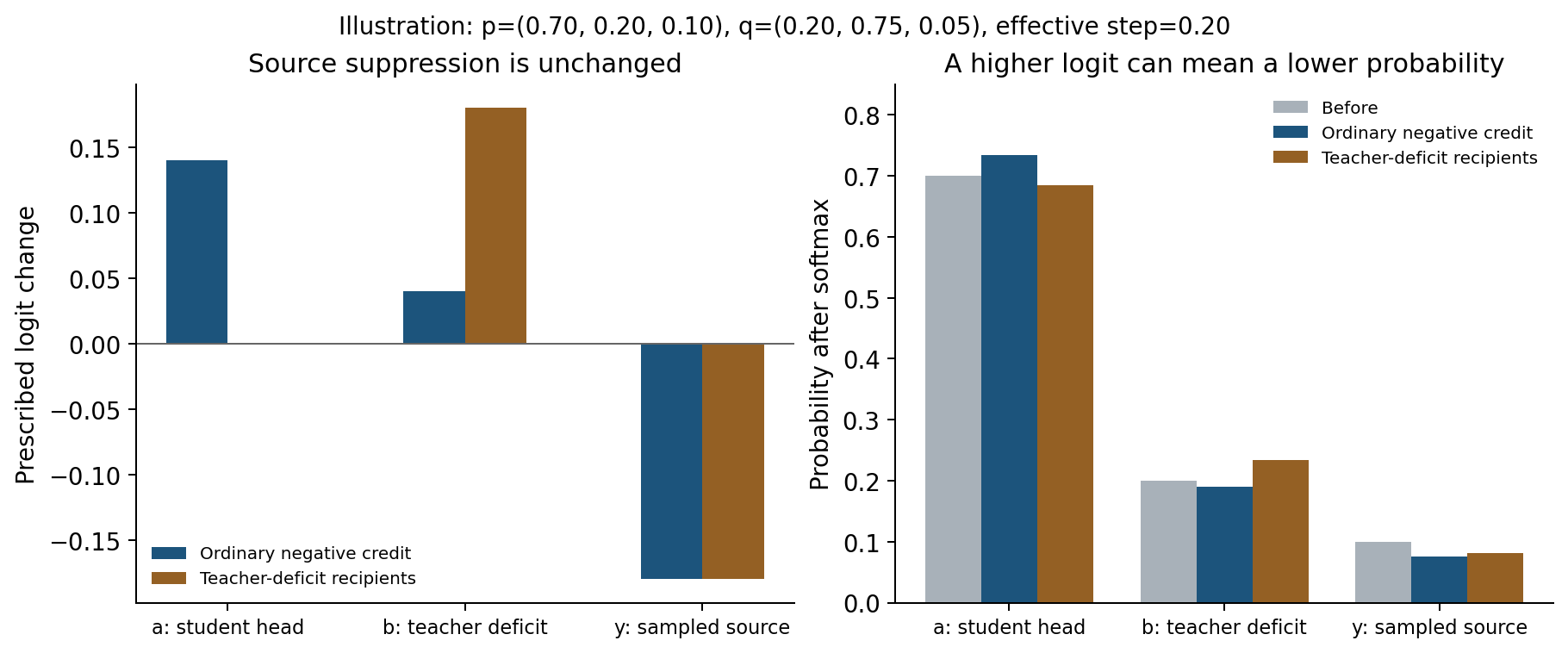
This raises $b$, the candidate the teacher favors. The final probability of $y$ differs between the two updates, however, despite its identical logit decrease. We control the logit signal; this example does not precisely transport an equal amount of probability mass.

The figure and table are worked examples of directly updating three logits, rather than measured parameter updates in a language model. In a real network, the signal passes through the model Jacobian, is aggregated across positions, and enters the optimizer. RouteOPD explicitly incorporates the teacher’s source–destination preferences into a pairwise objective. Our later experiment tests a different prototype for negative-feedback backpropagation, rather than reproducing that paper.

2.4 How OPD Layers Teacher Preferences onto the Squeezing Effect

OPD has two mechanisms operating together: softmax competition within each negative-feedback update, and teacher supervision across samples. The former allocates the recipient signal according to the student distribution; the latter adjusts the sign and magnitude of the signal through each candidate’s teacher gap.

Still at a fixed prefix, under purely on-policy sampling and without clipping, let each candidate’s signal be $A_j=\log q_j-\log p_j$. Taking the expectation over every possible sampled token gives

$$\mathbb E_{y\sim p}[A_y(e_y-p)] =p\odot\left(A-\mathbb E_p A\right) =-\nabla_z D_{\mathrm{KL}}(p\|q).$$

The example above examines a single negative signal after sampling $y$. Sampling $b$, which the teacher favors, instead gives a positive signal. Averaged across samples, ordinary OPD’s local expected update raises $b$. Teacher preferences enter the expected update through different candidates’ gaps, while student preferences appear in the competitive structure of each sampled update.

This clarifies the role of explicit routing: it places teacher preferences directly into the recipient direction of a particular negative-feedback update, actively selecting recipients under finite sampling. Ordinary OPD already has teacher supervision; routing changes how that supervision is used within an individual update.

OPSA provides evidence from the other side. Its teacher-independent updates yield gains in several settings, showing that reshaping the student’s existing distribution and suppressing tail patterns has learning value in itself. Teacher supervision and the reorganization of the student distribution can both contribute, affecting the introduction of new preferences and competition among existing preferences, respectively.

2.5 Teacher Routing: A Promising Direction for Further Research

Giving the teacher control over recipient preferences is a natural algorithmic direction for the squeezing effect. Since a few positions carry most of the updates, their recipient directions deserve deliberate design, allowing the teacher’s relative preferences among candidates to enter the update directly.

RouteOPD already reports positive experimental results. Across four teacher–student settings, its mean accuracy over four mathematical benchmarks improves by 2.19–3.61 percentage points over sampled-RKL OPD, with an average gain of 2.70 percentage points across settings. It pairs student probability surpluses with teacher probability deficits, then constructs a pairwise log-odds objective using a shared, bounded teacher potential, together with Huber loss and an adaptive budget. The teacher’s recipient preferences, objective form, and update strength work together in this design.

We also built a more direct backpropagation prototype on EOPD. It retains the sampled teacher gap, PPO clipping, and positive-signal branch, replacing the recipient direction only in the negative-signal branch with $(q-p)_+$ within the teacher’s top16 candidates. The prototype preserves source suppression and the direct score gradient of stop tokens. It tests one implementation of keeping the credit signal while changing the recipient direction. This and RouteOPD’s pairwise objective with an adaptive budget are different algorithmic implementations.

The prototype achieved 67.90% MATH500 Avg@8, compared with 68.275% for the EOPD baseline; their Pass@8 scores were 86.40% and 87.60%, respectively. The complete setup and results by question are documented in the experiment record. These initial results provide a reusable starting point for comparing recipient rules, routing budgets, and the positions where routing is applied. RouteOPD’s positive results support further work on turning teacher preferences into effective updates.

Three concrete questions remain:

• Design position selection and recipient direction together. Use high entropy, large gradients, or IER to select useful, reliable positions, then introduce teacher recipient preferences at those positions. Sparse supervision can address both where to learn and which candidates to favor.
• Adapt routing strength to the teacher’s needs. The size, concentration, and uncertainty of teacher deficits can jointly determine the budget, matching update magnitude to the distributional differences that need correction.
• Compare objective forms. Modifying backward directly, fitting pairwise log-odds, and adding conditional FKL each express teacher preferences through different learning geometries. Their interactions with PPO constraints and the optimizer deserve systematic comparison.

Sparse updates answer which positions to learn at; teacher routing answers which candidates to favor. Together, they concentrate a limited learning budget at critical positions and use teacher preferences to shape competition there. This is where the two observations in this article meet in algorithm design.

The two conclusions we retain are clear: a few tokens can carry training because the effective update budget is already highly concentrated; when negative feedback suppresses a token, softmax competition amplifies the existing ranking among the student’s remaining candidates. Teacher supervision then influences that competition through candidate-specific learning signals or explicit recipient directions. The first perspective explains why updates are sparse; the second explains how updates shape preferences.

---

Data and verification materials: raw per-token data, entropy–probability overlap analysis, and complete comparison results. The numerical inputs and generation code for both figures are saved; the plotting script reproduces them. The materials archive includes the required data and directory structure.

Data notes: the 256 positions come from 8 short arithmetic rollouts. The early loader used BF16 parameters; embedding–output-head weight tying was restored in subsequent formal training. Budget statistics sum individual-token contribution lengths; the top-20% quantile threshold selects 52 positions. Entropy describes the full distribution, while sampled probability describes the token actually drawn; this article reports the measured overlap among the three selectors in this dataset. The routing experiment uses a custom backward, retaining the original sampled loss value for diagnostics, and task performance is evaluated independently for a single seed.